How to use the Offset Function in MS Excel as a Data Analyst

How to use the Offset Function in MS Excel as a Data Analyst

Part 1: Introduction

Part 2: Where to use this?

Part 3: The OFFSET Formula explained

Part 4: Practical Example

PART 1: Introduction

• OFFSET tells Microsoft Excel to “fetch” a cell location from within a data range.
• It enables you to return a result from a specific cell or range of cells that has a specified number of rows and columns, away from the cell you have specified.
• The OFFSET function is part of the Lookup and Reference group of functions in Excel.

PART 2: Where to use this

• We have 2 sets of values, the main values, and each main value has a subset of values.
• If we pick a main value, we want Excel to automatically show us the subset values that correspond to the main value we picked.
• Case 1: As the data analyst, management wants to see the performance of each sales rep in the team, and it happens that each sales rep functions in different states, and you want to call up their sales per product in each state.
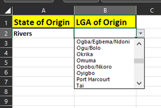
• Case 2: You want the user that is filling the online form, to select a particular State, the next part of the form should only show LGAs that correspond to the State selected.
• Case 3: A library with sections, and each section has a list of books. When a reader request for the books in a section, the OFFSET Function can be used to lookup only the books in that section.
• CASE 4: A supermarket where the range of products available for a section can be called up easily and dynamically.

PART 3: The OFFSET Formula looks like this 👇👇👇

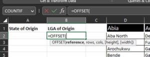
=OFFSET(reference, rows to move, columns to move, height, width)

1. Reference.

The first part of the syntax is the reference argument. The reference argument is the starting cell from where you want to go X rows down/up or Y columns right/left.

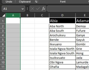
For the example we will use in the practical section, the starting point in the referenced cell is (ABIA).

2. Row.

The rows argument tells the OFFSET function the vertical location of the range you want to return (down/up).

In this example, we want to return the value 1 row below the starting reference (ABA NORTH). 

3. Column.

The columns argument tells the OFFSET function the horizontal location of the range you want to return. In this example, since we want to lookup the data, we use the MATCH function in place of col.

MATCH looks for a value and returns the row number of the found value to the OFFSET function. The MATCH function has 3 arguments

• Lookup value: a cell reference to the value you want to look for (the lookup value).

In the example, click the cell at the far left where the state will by referenced, and fix it using F4.

• Lookup array: The lookup array is the column where you want to search for the lookup value.

In the example, this is all the states we have, and fix it with F4.

• Match type: The last argument of the MATCH function determines which type of match you want. The match type can be -1, 0, 1.

In the example, use 0 to get the exact match.

Also since offset and match have a difference of -1, close the MATCH bracket with -1.

4/5. Height and Width.

The height and width arguments are only used to return a range of multiple adjacent cells.

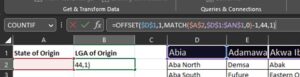
In this example, the height represents the product or state with the highest component. Kano has 44 LGA, so use 44.

In this example, set the width to 1.

PART 4: Practical example

To follow along with this tutorial, download the sample data set here.

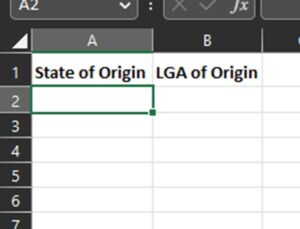
Step 1: Copy the dataset and place on a new worksheet (SHEET 2)

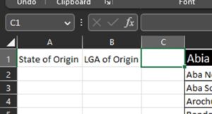
Step 2: Insert 3 columns at the beginning.

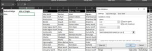
Step 3: Rename the headers (State of Origin, LGA of Origin)

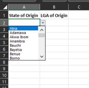
Step 4: Use data validation to create the cell reference to the value you want to look for (the lookup value). Click on A2

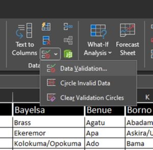
Go to Data, Data Tools, Data Validation

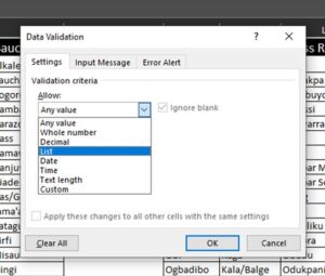
In settings, set Allow to LIST

Set the source. Select the names of the states.

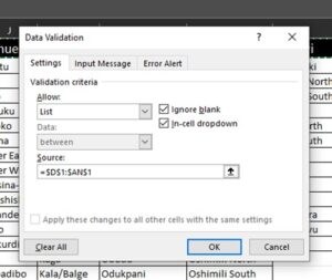
Click ok.

Join our Data Analytics class

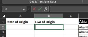
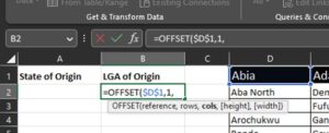
Step 5: Start the offset. Select B2

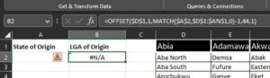
Step 6: Write the OFFSET formula

Step 7: Pick the reference argument. This is the starting cell from where you want to get values. D1. Fix it using F4, $D$1.

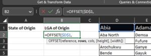
Step 8: Set the row to 1.

Step 9: type MATCH

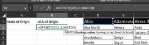
Step 10: Select the lockup cell and fix it. $A$2

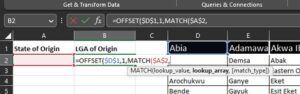
Step 11: Select the lookup array, and fix it. $D$1:$AN$1

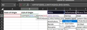
Step 12: Set the match type to 0. Close the bracket. Type -1.

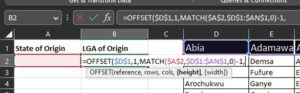
Step 13: Set the height to 44, and the width to 1.

Hit enter

Select a state, and the values will change

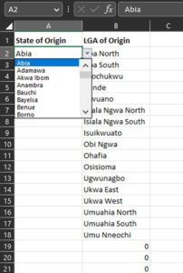
Step 14: Use data validation to turn the LGA into a dropdown list.

Cut the formula, click on another cell, click again on the main cell (B2), go to data validation and paste the formula in the source section.

The LGA now appear as a drop down list

Join our Data Analytics class